This page outlines the processing of DCT, where we quantize the DCT components. It converts to a Gray scale image, and then applies a quantization matrix:
Quantization in DCT |
Theory
JPEG is an excellent compression technique which produces lossy compression (although in one mode it is lossless). As seen from the previous chapter, it has excellent compression ratio when applied to a color image. This chapter introduces the JPEG standard and the method used to compress an image. It also discusses the JFIF file standard which defines the file format for JPEG encoded images. Along with GIF files, JPEG is now one of the most widely used standards for image compression.
JPEG coding
JPEG is a typical standard for image compression has been devised by the Joint Photographic Expert Group (JPEG), a subcommittee of the ISO/IEC, and the standards produced can be summarized as follows:
It is a compression technique for gray-scale or color images and uses a combination of dis-crete cosine transform, quantization, run-length and Huffman coding.
It has resulted from research into compression ratios and the resultant image quality. The main steps are:
- Data blocks. Generation of data blocks
- Source-encoding. Discrete cosine transform and quantization
- Entropy-encoding. Run-length encoding and Huffman encoding
Unfortunately, compared with GIF, TIFF and PCX, the compression process is relatively slow. It is also lossy in that some information is lost in the compression process. This infor-mation is perceived to have little effect on the decoded image.
GIF files typically take 24-bit color information (8 bits for red, 8 bits for green and 8 bits for blue) and convert it into an 8-bit color palette (thus reducing the number of bits stored to approximately one-third of the original). It then uses LZW compression to further reduce the storage. JPEG operates differently in that it stores changes in color. As the eye is very sensi-tive to brightness changes and less on color changes, then if these changes are similar to the original then the eye perceives the recovered image as very similar to the original.
Color conversion and subsampling
The first part of the JPEG compression separates each color component (red, green and blue) in terms of luminance (brightness) and chrominance (color information). JPEG allows more losses on the chrominance and less on the luminance as the human eye is less sensitive to color changes than to brightness changes. In an RGB image, all three colors carry some brightness information but the green component has a stronger effect on brightness than the blue component.
typical scheme for converting RGB into luminance and color is CCIR 601, which con-verts the components into Y (can be equated to brightness), Cb (blueness) and Cr (redness). The Y component can be used as a black and white version of the image.
Each component is computed from the RGB components as:
Y=0.299R+0.587G+0.114B
Cb=0.1687R–0.3313G+0.5B
Cr=0.5R–0.4187G+0.0813B
For the brightness (Y) it can be seen that green has the most effect and blue has the least effect. For the redness (Cr), the red color (of course) has the most effect and green the least. For blueness (Cb), the blue color has the most effect and green the least. Note that the YCbCr components are often known as YUV (especially in TV systems).
subsampling process is then samples the Cb and Cr components at a lower rate than the Y component. A typical sampling rate is four samples of the Y component for a single sample of the Cb and Cr components (4:1:1). This sampling rate is normally set with the compression parameters, the lower the sampling, the smaller the compressed data and the shorter the compression time. The JPEG header contains all the information necessary to properly decode the JPEG data.
DCT coding
The DCT (discrete cosine transform) converts intensity data into frequency data, which can be used to tell how fast the intensities vary. In JPEG coding the image is segmented into 8x8 pixel rectangles, as illustrated in Figure 8.1. If the image contains several components (such as Y,Cb,Cr or R,G,B), then each of the components in the pixel blocks is operated on sepa-rately. If an image is subsampled, there will be more blocks of some components than of others. For example, for 2x2 sampling there will be four blocks of Y data for each block of Cb or Cr data.
The data points in the 8x8 pixel array starts at the upper right at (0,0) and finish at the lower right at (7,7). At the point (x,y) the data value is f(x,y). The DCT produces a new 8x8 block (uxv) of transformed data using the formula:
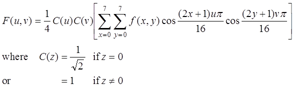
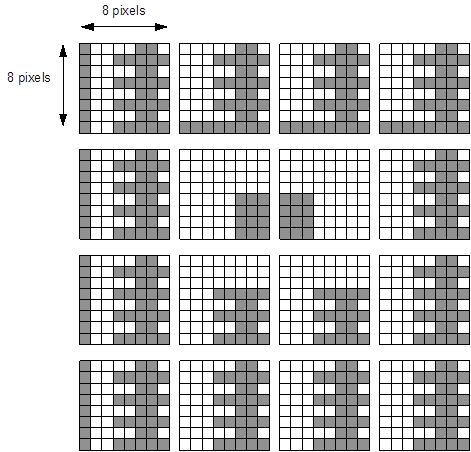
Figure 1 Segment of an image in 8x8 pixel blocks
This results in an array of space frequency F(u,v) which gives the rate of change at a given point. These are normally 12-bit values which give a range of 0 to 1024. Each component specifies the degree to which the image changes over the sampled block. For example:
- F(0,0) gives the average value of the 8x8 array.
- F(1,0) gives the degree to which the values change slowly (low frequency).
- F(7,7) gives indicates the degree to which the values change most quickly in both directions (high frequency).
The coefficients are equivalent to representing changes of frequency within the data block. The value in the upper left block (0,0) is the DC or average value. The values to the right of a row have increasing horizontal frequency and the values to the bottom of a column have increasing vertical frequency. Many of the bands though, end up having zero, or almost zero terms.
The program below gives a C program which determines the DCT of an 8x8 block and Sample run 1 shows a sample run with the resultant coefficients.
#include	<stdio.h>
#include	<math.h>
#define	PI	3.1415926535897

int	main(void)
{
int	x,y,u,v;
float	in[8][8]=	{{144,139,149,155,153,155,155,155},
				{151,151,151,159,156,156,156,158},
				{151,156,160,162,159,151,151,151},
				{158,163,161,160,160,160,160,161},
				{158,160,161,162,160,155,155,156},
				{161,161,161,161,160,157,157,157},
				{162,162,161,160,161,157,157,157},
				{162,162,161,160,163,157,158,154}};
float	out[8][8],sum,Cu,Cv;

	for (u=0;u<8;u++)
	{
		for (v=0;v<8;v++)
		{
			sum=0;
			for (x=0;x<8;x++)
				for (y=0;y<8;y++)
				{
					sum=sum+in[x][y]*cos(((2.0*x+1)*u*PI)/16.0)*
						cos(((2.0*y+1)*v*PI)/16.0);
				}
			if (u==0) Cu=1/sqrt(2); else Cu=1;
			if (v==0) Cv=1/sqrt(2); else Cv=1;

			out[u][v]=1/4.0*Cu*Cv*sum;
			printf("%8.1f ",out[u][v]);
		}
		printf("\n");
	}
	printf("\n");
	return(0);
}
The program uses a fixed 8x8 block of:
144	139	149	155	153	155	155	155
151	151	151	159	156	156	156	158
151	156	160	162	159	151	151	151
158	163	161	160	160	160	160	161
158	160	161	162	160	155	155	156
161	161	161	161	160	157	157	157
162	162	161	160	161	157	157	157
162	162	161	160	163	157	158	154
Sample run 8.1
  1257.9      2.3     -9.7     -4.1      3.9      0.6     -2.1      0.7
   -21.0    -15.3     -4.3     -2.7      2.3      3.5      2.1     -3.1
   -11.2     -7.6     -0.9      4.1      2.0      3.4      1.4      0.9
    -4.9     -5.8      1.8      1.1      1.6      2.7      2.8     -0.7
     0.1     -3.8      0.5      1.3     -1.4      0.7      1.0      0.9
     0.9     -1.6      0.9     -0.3     -1.8     -0.3      1.4      0.8
    -4.4      2.7     -4.4     -1.5     -0.1      1.1      0.4      1.9
    -6.4      3.8     -5.0     -2.6      1.6      0.6      0.1      1.5
Notice that the values of the most significant values are in the top left-hand corner and that many terms are near to zero. It is this property which allows many values to become zeros when quantized. These zeros can then be compressed using run-length coding and Huffman codes.
Quantization
The next stage of the JPEG compression is quantization where bias is given to lower-frequency components. JPEG divides each of the DCT values by a quantization factor, which is then rounded to the nearest integer. As the DCT factors are 8x8 then a table of 8x8 of quantization factors are used, corresponding to each term of the DCT output. The JPEG file then stores this table so that the decoding process may use this table or a standard quantization table. Note that files with multiple components must have multiple tables, such as one each for the Y, Cb and Cr components.
For example the values of the quantized high-frequency term (such as F(7,7)) could have a term of around 100, while the low-frequency term could have a factor of 16. These values define the accuracy of the final value. When decoding, the original values are (approximately) recovered by multiplying by the quantization factor.
Figure 2 shows that, for a factor of 100, the values between 50 and 150 would be quantized as a 1, thus the maximum error would be +/-50. The maximum error for the factor of 16 is +/-8. Thus the maximum error of the final unquantized value for a scale factor of 100 is 1.22% (5000/4096), while a factor of 16 gives a maximum error of 0.20% (800/4096). So, using the factors of 100 for F(7,7) and 16 for F(0,0), and a 12-bit DCT, the F(0,0) term would range from 0 to 256 and the F(7,7) term would range from 0 to 41. The F(0,0) term could be coded with 8 bits (0 to 255) and the F(7,7) term with 6 bits (0 to 63).
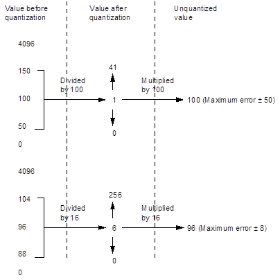
Figure 2 Example of quantization
Program 2 normalizes and quantizes (to the nearest integer) the example given previously. To recap, the input 8x8 block is:
144	139	149	155	153	155	155	155
151	151	151	159	156	156	156	158
151	156	160	162	159	151	151	151
158	163	161	160	160	160	160	161
158	160	161	162	160	155	155	156
161	161	161	161	160	157	157	157
162	162	161	160	161	157	157	157
162	162	161	160	163	157	158	154
The applied normalization matrix is:
5		3		4		4		4		3		5		4
4		4		5		5		5		6		7		12
8		7		7		7		7		15		11		11
9		12		13		15		18		18		17		15
20		20		20		20		20		20		20		20
20		20		20		20		20		20		20		20
20		20		20		20		20		20		20		20
20		20		20		20		20		20		20		20
Program 2
#include	<stdio.h>
#include	<math.h>
#define	PI	3.1415926535897

int	main(void)
{
int	x,y,u,v;
float	in[8][8]=	{
		{144,139,149,155,153,155,155,155},
		{151,151,151,159,156,156,156,158},
		{151,156,160,162,159,151,151,151},
		{158,163,161,160,160,160,160,161},
		{158,160,161,162,160,155,155,156},
		{161,161,161,161,160,157,157,157},
		{162,162,161,160,161,157,157,157},
		{162,162,161,160,163,157,158,154}};

float	norm[8][8]=	{
	{5,3,4,4,4,3,5,4},
	{4,4,5,5,5,6,7,12},
	{8,7,7,7,7,15,11,11},
	{9,12,13,15,18,18,17,15},
	{20,20,20,20,20,20,20,20},
	{20,20,20,20,20,20,20,20},
	{20,20,20,20,20,20,20,20},
	{20,20,20,20,20,20,20,20}};

int	out[8][8];
float	sum,Cu,Cv;

	for (u=0;u<8;u++)
	{
		for (v=0;v<8;v++)
		{
			sum=0;
			for (x=0;x<8;x++)
				for (y=0;y<8;y++)
				{
					sum=sum+in[x][y]*cos(((2.0*x+1)*u*PI)/16.0)*
						cos(((2.0*y+1)*v*PI)/16.0);
				}
			if (u==0) Cu=1/sqrt(2); else Cu=1;
			if (v==0) Cv=1/sqrt(2); else Cv=1;

			out[u][v]=(int)1/4.0*Cu*Cv*sum/norm[u][v];
			printf("%8d ",out[u][v]);
		}
		printf("\n");
	}

	printf("\n");
	return(0);
}
Source code
The following outlines the Python code used:
"""
Simulation of basic JPEG compression,
only DCT + quantization IDCT,
not including entropy-encoding/Huffman-coding
"""

# jpeggraysim.py
import cv2
import numpy as np
import os

import  sys

matrix = "[  [16,  11,  10,  16,  24,  40,  51,  61],  [12,  12,  14,  19,  26,  58,  60,  55],  [14,  13,  16,  24,  40,  57,  69,  56],  [14,  17,  22,  29,  51,  87,  80,  62],  [18,  22,  37,  56,  68, 109, 103,  77],  [24,  35,  55,  64,  81, 104, 113,  92],  [49,  64,  78,  87, 103, 121, 120, 101],  [72,  92,  95,  98, 112, 100, 103,  99]]"

file ='1111'
type=0

if (len(sys.argv)>1):
        file=str(sys.argv[1])

if (len(sys.argv)>2):
        type=int(sys.argv[2])

if (len(sys.argv)>3):
        matrix=str(sys.argv[3])

std_luminance_quant_tbl = eval(matrix)

def JPEG_DCT(imgfile, file,type):
    # 1 channel x 8 bits, grayscale
    img = cv2.imread(imgfile,0)

#    wndName = "original grayscale"
#    cv2.namedWindow(wndName, cv2.WINDOW_AUTOSIZE)
#    cv2.imshow(wndName, img)

    iHeight, iWidth = img.shape[:2]
#    print "size:", iWidth, "x", iHeight

    # set size to multiply of 8
    if (iWidth % 8) != 0:
        filler = img[:,iWidth-1:]
        #print "width filler size", filler.shape
        for i in range(8 - (iWidth % 8)):
            img = np.append(img, filler, 1)

    if (iHeight % 8) != 0:
        filler = img[iHeight-1:,:]
        #print "height filler size", filler.shape
        for i in range(8 - (iHeight % 8)):
            img = np.append(img, filler, 0)

    iHeight, iWidth = img.shape[:2]


    # array as storage for DCT + quant.result
    img2 = np.empty(shape=(iHeight, iWidth))

    # FORWARD ----------------
    # do calc. for each 8x8 non-overlapping blocks

    for startY in range(0, iHeight, 8):
        for startX in range(0, iWidth, 8):
            block = img[startY:startY+8, startX:startX+8]

            # apply DCT for a block
            blockf = np.float32(block)     # float conversion

            dst = cv2.dct(blockf)          # dct

            if (startY==0 and startX==0):
		dctval=dst

            # quantization of the DCT coefficients
            blockq = np.around(np.divide(dst, std_luminance_quant_tbl))
            blockq = np.multiply(blockq, std_luminance_quant_tbl)

            # store the result
            for y in range(8):
                for x in range(8):
                    img2[startY+y, startX+x] = blockq[y, x]

    block1 = img[0:8, 0:8]
    print "Before (1st block):\n",block1
    print "DCT(1st block):\n",np.int32(dctval)
    block1 = img2[0:8, 0:8]
    print "After (1st block):\n",block1

    # INVERSE ----------------
    for startY in range(0, iHeight, 8):
        for startX in range(0, iWidth, 8):
            block = img2[startY:startY+8, startX:startX+8]

            blockf = np.float32(block)     # float conversion
            dst = cv2.idct(blockf)         # inverse dct
            np.place(dst, dst>255.0, 255.0)     # saturation
            np.place(dst, dst<0.0, 0.0)         # grounding
            block = np.uint8(np.around(dst))

            # store the results
            for y in range(8):
                for x in range(8):
                    img[startY+y, startX+x] = block[y, x]

    block1 = img[0:8, 0:8]
    print "Reverse (1st block):\n",block1

    file1 = "c:\\inetpub\\wwwroot\\log\\"+file+".jpg"
    cv2.imwrite(file1,img)

    print "Image Size:", iWidth, "x", iHeight
    b = os.path.getsize(file1)
    print "File size:",b

#    wndName1 = "DCT + quantization + inverseDCT"
#    cv2.namedWindow(wndName1, cv2.WINDOW_AUTOSIZE)
#    cv2.imshow(wndName1, img)
#    file = "c:\\inetpub\\wwwroot\\log\\"+file+".jpg"
#

#    cv2.waitKey(0)
#    cv2.destroyWindow(wndName1)
#    cv2.destroyWindow(wndName)

JPEG_DCT("c:\\python27\\mini.jpg",file,type)